Tuesday, 27 December 2016

Deep learning as new electronics


It is hard to imagine a modern life without electronics: radios, TVs, microwaves, mobile phones and many more gadgets. Dump or smart, they are all based on the principles of semi-conducting and electromagnetism. Now we are using these devices for granted without worrying about these underlying laws of physics.  Most people do not care about circuits that run in chips and carry out most functions of the devices.

For the past 5 years, a new breed of human-like functionalities has emerged through advances of a new field called deep learning: self-driving cars, voice command in mobile phone, translation in hundreds of language pairs and a new kind of art. In 2016, ten years after its revival, deep learning has taken over the Internet. People have used deep learning-powered products in daily life without worrying about how the underlying neural nets work.

These two fields free us from many physical and psychological constraints:

  • Electronic devices give us freedom of communication over distance, a new kind of experiences with augmented reality and many more.
  • Deep learning enables freedom from having to make tedious and incorrect decisions (e.g., driving a car), freedom of information access (personalization), of hand (e.g., voice command), of finance (automated trading), of feature extraction (through representation learning), and many more.
It is worth noting that electronics and deep learning are different in principles.
  • Electronics devices are designed with great precision for specific functions in mind. Imprecision comes from the quantum uncertainty principle and thermal fluctuations.
  • Neural nets on the other hand, are designed to learn to perform a function of its own, where data (and sometimes model) uncertainty is built in.
However, it is also striking that they are quite similar in many ways.

Super-city of interconnected simple parts

Modern electronic devices are truly super-cities built out of just few kinds of primitive building blocks. The same holds for deep neural nets:
  • Electronic primitives: resistor, capacitor, transistor, coil, diode, logic gate and switch.
  • Neural net primitives: integrate-and-fire neuron, multiplicative gating, differentiable logic gate, switch and attention module. Interestingly, one of the most recent idea is called "Highway networks", borrowing the idea that highway traffic is free of traffic lights.
These primitives are connected in graphs:
  • Electronic devices works by moving electrons in correct order and number. The force that makes them move is potential difference. A design circuit captures all necessary information.
  • In neural nets, the activation function is like the electronic current. The main difference is that the magnitude of "current" in neural nets can be learnt. A computational graph is what is needed for model execution.
Not just analogy: A two-way relationship
  • Electronics deep learning: At present, advances in electronics have given huge boost in efficiency of deep learning with GPU, TPU and other initiatives. It is interesting to see if we can learn from electronics in designing deep nets? For example, will something analogous to integrated-circuits in deep architectures?
  • Deep learning  electronics: I predict that soon the reverse will hold true: deep learning will play a great role in improving efficiency and functionalities of electronic devices. Stay tuned.
Sunday, 25 December 2016

Making a dent in machine learning, or how to play a fast ball game


Neil Lawrence had an interesting observation about the current state of machine learning, and linked it to fast ball games:
“[…] the dynamics of the game will evolve. In the long run, the right way of playing football is to position yourself intelligently and to wait for the ball to come to you. You’ll need to run up and down a bit, either to respond to how the play is evolving or to get out of the way of the scrum when it looks like it might flatten you.”
Neil Lawrence is known for his work in Gaussian Processes and is a proponent of data efficiency. He used to be professor at University of Sheffield, is now with Amazon. Apparently the strategy works. The ball has come to him.

I once heard about a professor who said he would come to top conferences just to learn what others were busy doing and tried to do something else.

I also read somewhere from a top physicist that students who applied to work with him often expressed the wish to study shiny-and-clean fields. Some other fields were too messy and seemed unsexy. The professor insisted that the messy fields were exactly the best to work on.

In "Letters to a young scientist", Edward Osborne Wilson told his life story. He spent his entire life cataloging ants since childhood, right at the time where ant ecology wasn't a shiny field. He is considered as father of biodiversity.

Wonder what to do in deep learning now?

It is an extremely fast ball game with thousands of top players. You will be either crushed with ideas being stolen weekly, or out of steam pretty quickly.

It looks like most of the low hanging fruits have been picked.

Then ask yourself, what is your unique position? What are your strengths and advantages that people do not have? Can you move faster than others? It may be by having access to data, access to expertise in the neighborhood, or borrowing angles outside the field. Sometimes digging up old ideas is highly beneficial, too.

Alternatively, just calm down, and do boring-but-important stuffs. Important problems are like the goal areas in ball games. The ball will surely come.

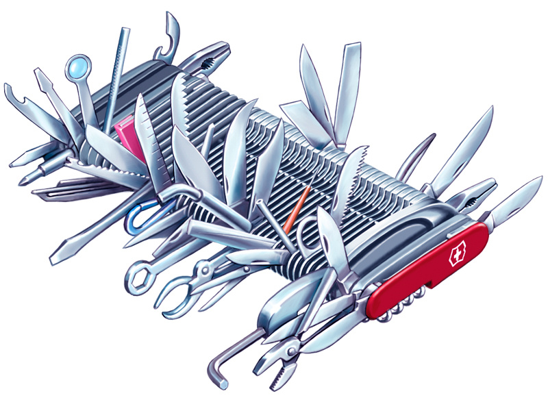
30 years of a Swiss army knife: Restricted Boltzmann machines


I read somewhere, but cannot recall exactly who said so, that in ancient worlds, 30 years are long enough for the new generation to settle down with a new system, regime or ideology. As there are only a few days away from 2017, I would like to look back the history of a 30-year old model which has captured my research attention for the past 10 years.

To some of you, restricted Boltzmann machine (RBM) may be a familiar name, especially for those who follow the current deep learning literature since the beginning. But RBM has also passed its prime time, so you may have heard about it in passing.

I was attracted to RBM for several reasons. When I was studying conditional random fields in 2004 and was looking for a fast way to train with arbitrary structures, Contrastive Divergence (CD) appears to be an interesting one. While CD is a generic technique, it was derived especially for RBMs. Second, RBM has "Boltzmann" in the name, which is kind of interesting, because physicists are kind of sexy :)

Needless too say, another big reason is that RBM, together with its cousin, Autoencoder are building blocks of unsupervised deep nets, which started the current revolution -- deep learning.

The greatest reason is that I think RBM is one of the most important classes of data models known to date, perhaps comparable to PCA in dimensionality-reduction  and k-means in clustering in terms of usefulness.

First introduced in 1986 by  Paul Smolensky under the name Harmonium in a classic two-volume book known as PDP (Parallel Distributed Processing), co-edited by Rumelhart and McLelland. RBMs were subsequently popularised by Geoff Hinton in the 2000s, especially in 2001 with the introduction of Contrastive Divergence (CD), and  in 2006 with the introduction of a deep version known as Deep Belief Nets (DBN).

Statistically, RBM is a probabilistic model of data, i.e., it assigns a probability (or density) to a multivariate data. Initially, RBMs are limited to binary data (known as Bernoulli-Bernoulli RBM), but subsequently extended to Gaussian data (known as Gaussian-Bernoulli RBM), and mixed-types (known as Mixed-variate RBM, or Thurstonian Boltzmann machine).

Source: http://deeplearning.net/tutorial/_images/rbm.png

RBM is a special case of Boltzmann machine, which is in turn a special case of Markov random field. It has two layers, one for observed data, the other for latent representation. Due to its special bipartite structure, MCMC inference can be implemented in a block-wise fashion. Learning is relatively fast with CD or its Persistent version. Estimating of latent representation is very fast with a single matrix operation. RBM is also a powerful model in the sense that it can represent any distribution given enough hidden units. As a Markov random field, it has log-linear paramerization which makes it easy to incorporate a variety of domain knowledge.

With all of these advantages, RBMs have been used successfully in many applications, ranging from density modelling, feature extraction, dimensional reduction, clustering, topic modeling, imputation, classification, retrieval and anomaly detection.

Some bias selection of developments
  • 1986: first introduced as Harmonium.
  • 2001: fast approximate biased learning introduced as Contrastive Divergence (CD)
  • 2004: generalized Harmonium introduced
  • 2006: used successfully in Deep Belief Networks
  • 2007: demonstrated with great success on a very large-scale task within the Netflix challenge
  • 2007: temporal RBM
  • 2008: recurrent temporal RBM
  • 2008: classification RBM
  • 2008: persistent CD introduced, essentially another variant of Young's.
  • 2008: convolutional RBMs
  • 2008: universality property proved
  • 2009: topic models with Replicated Softmax
  • 2009: matrix modelling with non i.i.d. RBMs, ordinal data, semi-restricted RBM
  • 2009: implicit mixtures of RBMs
  • 2010: factored high-order RBM
  • 2010: mean-covariance RBM
  • 2010: rectifier linear units RBM
  • 2010: deep BM
  • 2011: mixed-variate RBM
  • 2012: a proper modeling of ordinal matrix data
  • 2013: Thurstonian BM for joint modeling of most known data types
  • 2013: nonnegative RBMs for parts-based representation
  • 2015: trained with graph priors, demonstrating better generalization
  • 2015: extended to tensor-objects
  • 2016: infinite RBM
In short, most of the work has been on extending the representational power of RBM to suit problem structures. The rest is about analysing theoretical properties of RBMs, making deep nets out of RBMs, and improving training speed & accuracy. For the past few years, research about RBMs has slowed down significantly, mostly because the superb accuracy of supervised deep nets, and the ease of deployment of deterministic nets on large-scale problems. 

Some of our own work

Thursday, 22 December 2016

Machine learning in three lines


How can we characterize machine learning as a field? What make machine learning work?

Machine learning is a fast changing field. The list of ideas is practically endless: Decision trees, ensemble learning, random forests, boosting, neural networks, hidden Markov models, graphical models, kernel methods, conditional random fields, sparsity, compressed sensing, budgeted learning, multi-kernel learning, transfer learning, co-training, active learning, multitask learning, deep learning, lifelong learning and many more.

The problem is, ideas come and go, and bounce back, roughly every 10-15 years. Long enough for a grad student learns the tricks, makes a big noise, graduates when it is still hot and gets a good academic job,  IF he is lucky to start early in the cycle. Also long enough so that the new batch of students are not aware of the hot things of the previous wave. How familiar is "particle filtering" to you?
Popular in the late 1990s and early 2000s, particle filtering is a fast way to generate samples of state for a dynamic system when an observation is made.
When I started my grad training in 2004, I asked one of my supervisors on what hot topic I should focus on. He said, pick either graphical models or kernel methods (which meant SVM at the time). I picked graphical models, and then was given conditional random fields (CRFs) to work on. By the time I submitted my PhD thesis in early 2008, CRFs were largely gone. SVMs were gone a couple of years before that, just around the time neural nets bounced back under a new umbrella, deep learning, in 2006. It used to be all about convex loss functions (SVMs & CRFs), now everything is non-convex. Local minima? Doesn't matter, adaptive stochastic gradient descents such as Adagrad, Adam or RMSprop will find a really good one for you.

Applying machine learning is like flying commercial aircraft

Ever wanted to apply a technique to your problem? A sure way is to employ a PhD in machine learning! Packages available, but what are the correct ways to use, let alone the best way? Think about flying commercial aircrafts. There are hundreds of knobs to tune. There are even autopilot mode. We just need to have two human pilots: one to tune the right knob at the right time, and the other making sure that the correct things are being done.

Wanna use deep learning? You need to decide between: feedforward, recurrent, convolutional nets and any combination of these three. Will attention be used? How about memory? Which loss function? Embedding size? Optimizers and their parameters? and many many more.

I work with clinicians on clinical problems. At least two of them -- young, smart and highly motivated -- insisted to come over and observe how I do machine learning and learn to do it themselves. They claimed they could do Statra, R and sometimes Python. My boss was crossed. This is not how collaboration should work, right? You want to learn our art for free, then trash us?

But I told the boss, let them come.

They came and left, even more puzzled. I ended up doing the job I usually did and so did they.

Machine learning in three lines

I once delivered an internal talk on deep learning. My boss requested that I talked only about three things. Just three things. This bugged me a lot. But the trick actually worked.

Here I am trying to characterize the current state of machine learning in general and it should apply to deep learning. Machine learning works by:
  1. Having good priors of the problem at hand (80-90% gain)
  2. Accounting for data uncertainty and model uncertainty with ensemble and Bayesian methods. (1-5% gain)
  3. Reusing models when data/model redundancies are available (5-10% gain)
Priors are king

By "good priors", I meant several things:
  • Features that capture all meaningful signals from data. Getting good features are the job of feature engineering, which usually accounts for 80-90% of total effort in a machine learning project. Once you have good features, most modern classifiers will work just fine. Deep learning succeed partly because it solves this problem.
  • Problem structures are respected. For example, sequential data would suggest the use of Hidden Markov Models (HMM) or chain-like Conditional Random Fields (CRF). In deep learning, it reduces to architecture engineering!
  • Knowledge about the model class. E.g., will linearity be the dominant model? What are the expected complexity and nonlinearity? Will interpretability needed? What is about transparency? Is sparsity important? For neural nets, how many layers?  For SVMs, will one kernel type be enough?
  • Assumptions about data manifold. One well-studied phenomenon is the intrinsic low dimensionality of data embedded in a very high dimensional space. This is usually manifested through data redundancies. Another assumption is separation of classes, e.g., the region at the class boundary is usually sparse, but is very dense near the class examplars. This assumption essentially gives rise to semi-supervised learning.
  • Assumptions about the data spaceHow many data instances? Will characterizing the data variance enough? If yes then use PCA. What about factors of variation are the key? If yes then RBM perhaps helps.
Don't forget uncertainty

Even with a good prior, we would never be sure that our choices are correct. Model uncertainty is there and must be accounted for. A popular way is to use many (diverse) models, then employ model averaging, ensemble methods and Bayesian approach. Deep learning has dropout as one of the best tricks invented in the past 10 years. It works like wonder. Bayesian neural nets, which were studied in mid 1990s, is also back!

In fact, every single modern challenge was won by some ensemble, mostly gradient boosting by the time of this writing AND model blending. One of the best known example is the Netflix challenge, which was won by blending hundreds of models -- so complex that Netflix found it was useless to implement in practice.

Many are easier than one

I often told my 5-year old daughter: do one thing at a time. But by listening to me AND playing at the same time, she has already multi-tasked. Humans seem to learn better that way. We learn by making senses of many co-occurring feedback signals.

A key idea in recent machine learning is model reuse. It has many forms:

  • Domain adaption, which is about reusing previous model on similar domains with minimal changes.
  • Transfer learning, which is about reusing models on similar tasks with minimal changes. In neural nets, it is equivalent to not forgetting the old trained nets when learning a new concepts.
  • Multi-task learning, which is about learning more than ones correlated tasks at a time. The idea is that models can be partly shared among tasks, leading to less training data and less overfitting.
  • Lifelong learning, which is like continual version of transfer learning. Just like humans, we learn to do new things from birth to death, every single day! Popularized by Sebastian Thrun in mid 1990s, lifelong learning is now back in various forms: never-ending learning at CMU, reinforce learning in robotics and games at a various labs.
  • Multi-X, where X is substituted by view, modality, instance, label, output/outcome, target, type and so on.

Tuesday, 20 December 2016

Everything old is new again: Nested sequential models


Recently, multi-layer RNN architectures have been demonstrated to work better than single-layer versions. The Google's Neural Machine Translation machine, for example, has 8 layers of LSTMs as of Dec 2016.

The idea goes back to earlier days of multi-layer HMMs in the 1990s, which are special cases of Dynamic Bayesian Networks. These were then followed by multi-layer Conditional Random Fields (CRFs), which are also special case of Dynamic CRFs.

The idea is that higher layers represent more abstract semantics. In temporal sequences, one would expect that the "clock" of the upper layers is slower than that of the lower layers. But most existing work has to explicitly design the temporal resolution by hand.

Learning the temporal resolution automatically is an attractive idea. In 1998, Hierarchical HMM was introduced, here parent state is assumed to generate a child sequence, and each child in turn generates a grandchild subsequence and so forth. The network becomes nested. Learning and inference cost cubic time, which is prohibitive for long sequences.

A CRF counterpart is known as Hierarchical Semi-Markov CRF introduced by us in 2008.

Both HHMMs and HSCRFs are member of the Stochastic Context-Free Grammar family, which is known for its cubic time complexity.  Not just being slow, HHMMs and HSCRFs are hopeless in large-scale tasks that require many bits to represent the world.

Given the recent successes of RNNs (mostly LSTM and GRU) for sequential tasks, one would naturally ask whether we can achieve the same feat as in HHMMs, that is, the hierarchy is learnt automatically from data. It proves to be a difficult task, until very recently. Check this paper by Bengio's group for more detail. I'm very curious to see how the idea plays out in practice. Let's wait and see.

Work by us:
  • Hierarchical semi-Markov conditional random fields for deep recursive sequential data, Truyen Tran, Dinh Phung, Hung Bui, Svetha Venkatesh,  Artificial Intelligence, 2017. (Extension of the NIPS'08 paper).
  • MCMC for Hierarchical Semi-Markov Conditional Random Fields, Truyen Tran, Dinh Q. Phung, Svetha Venkatesh and Hung H. Bui. In NIPS'09 Workshop on Deep Learning for Speech Recognition and Related Applications. December, 2009, Whistler, BC, Canada.
  • Hierarchical Semi-Markov Conditional Random Fields for Recursive Sequential Data, Truyen Tran, Dinh Q. Phung, Hung H. Bui, and Svetha Venkatesh. In Proc. of 21st Annual Conference on Neural Information Processing Systems, Dec 2008, Vancouver, Canada. 
  • AdaBoost.MRF: Boosted Markov random forests and application to multilevel activity recognition, Truyen Tran, Dinh Quoc Phung, Hung Hai Bui, and Svetha Venkatesh. In Proc. of  IEEE Conference on Computer Vision and Pattern Recognition, volume Volume 2, pages 1686-1693, New York, USA, June 2006.

Monday, 19 December 2016

Everything old is new again: Deep statistical relational learning


In the age of combinatorial innovation, old things will be given a new shiny face, even nothing really new happens. The same holds for Statistical Relation Learning (SRL) -- a sub-field of machine learning for characterizing the relational structure of the world.

Started in late 1990s, SRL had gone through a fruitful period of about 10 years and reached its peak in 2007 with the publication of a book titled "Introduction to Statistical Relational Learning" co-edited by Lise Getoor and the late Ben Taskar (who died unexpectedly in 2013 at the age of 36 at his academic peak). Many significant models appeared in the first half of the 2000s, including Conditional Random Fields (CRF, 2001), Relational Markov networks (2002) and Markov Logic Networks (2006). Despite being more powerful than non-relational alternatives, SRL still relies on manual feature engineering, which will soon reach its limit of utility.

Developed rather in parallel is Deep Learning (DL), where the current wave officially started in 2006 with the publication of Deep Belief Networks in Science. Deep learning is concerned about learning data abstraction (aka features), favoring end-to-end learning through multiple steps of non-linear computation.

A combinatorial thinking would naturally lead to the question whether these two sub-fields can work together. The answer is a big YES, because SRL and DL are rather complementary. For example, in the past 3 years, there have been lots of papers marrying CRF and deep nets. While CRFs offer a semi-formal framework for joint learning and inference, deep nets offer learning of features (with feedforward nets), deterministic dynamics (with recurrent nets), and translation invariance (with convolutional nets). The marriage would be a happy one. But like any marriage of convenience, it won't go very far. Some genuine blending is needed.

Our recent work,  Column Networks, scheduled to appear in AAAI'17, blends the SRL and DL even further so that learning and inference can be carried out naturally. The term "column" refers to the famous columnar structure of neo-cortex in mammals. Interestingly, Column Networks share design features of all three main deep net architectures:

  • A column is a feedfoward net,
  • Parameters are tied across layers, which is essentially the idea behind recurrent nets.
  • The network between columns is designed so that the multi-relations between columns are invariant across columns, hence the translation invariance property of convolutional nets.
As Column Networks are very generic, expect more to come in the next few months. Stay tuned.

Updated references

  • Column Networks for Collective Classification, T Pham, T Tran, D Phung, S Venkatesh, AAAI'17.
  • Graph-induced restricted Boltzmann machines for document modeling, Tu D. Nguyen, Truyen Tran, D. Phung, and S. Venkatesh, Information Sciences. doi: 10.1016/j.ins.2015.08.023
  • Neural Choice by Elimination via Highway Networks, Truyen Tran, Dinh Phung and Svetha Venkatesh,  PAKDD workshop on Biologically Inspired Techniques for Data Mining (BDM'16), April 19-22 2016, Auckland, NZ.
  • Predicting delays in software projects using networked classification, Morakot Choetikertikul, Hoa Khanh Dam, Truyen Tran, Aditya Ghose, 30th IEEE/ACM International Conference on Automated Software Engineering, November 9–13, 2015 Lincoln, Nebraska, USA.
  • Learning vector representation of medical objects via EMR-driven nonnegative restricted Boltzmann machines (e-NRBM), Truyen Tran, Tu D. Nguyen, D. Phung, and S. Venkatesh, Journal of Biomedical Informatics, 2015, pii: S1532-0464(15)00014-3. doi: 10.1016/j.jbi.2015.01.012. 
  • Cumulative Restricted Boltzmann Machines for Ordinal Matrix Data Analysis, Truyen Tran, Dinh Phung and Svetha Venkatesh, in Proc. of. the 4th Asian Conference on Machine Learning (ACML2012), Singapore, Nov 2012.
  • Ordinal Boltzmann Machines for Collaborative Filtering. Truyen Tran, Dinh Q. Phung and Svetha Venkatesh. In Proc. of 25th Conference on Uncertainty in Artificial Intelligence, June, 2009, Montreal, Canada. 
  • Hierarchical Semi-Markov Conditional Random Fields for Recursive Sequential Data, Truyen Tran, Dinh Q. Phung, Hung H. Bui, and Svetha Venkatesh. In Proc. of 21st Annual Conference on Neural Information Processing Systems, Dec 2008, Vancouver, Canada.
  • AdaBoost.MRF: Boosted Markov random forests and application to multilevel activity recognition, Truyen Tran, Dinh Quoc Phung, Hung Hai Bui, and Svetha Venkatesh. In Proc. of  IEEE Conference on Computer Vision and Pattern Recognition, volume Volume 2, pages 1686-1693, New York, USA, June 2006.

Machine learning four years after the turning point


In May 2012 I wrote a note titled "Machine at its turning point" to argue for the new wave of machine learning in that we do not need to worry about having a convex loss but rather be happy with non-convex ones. At the time I did not know about AlexNet and its record-breaking result on the ImageNet benchmark. It was published 7 months later in NIPS'12.

AlexNet was truely a turning point for machine learning. It declared the winning of deep neural nets over others, which were combination of clever manual feature engineering and some variants of SVMs or random forests. AlexNet is remarkable in many ways: Dropout, rectifier linear units, end-to-end training on massive data with GPUs, data augmentation and carefully designed convolutional nets.

It was the year that Yann LeCun posted his complaints about the computer vision community, but quickly retracted his boycott given the aftershock of AlexNet.

Recently, there has been an interesting comment floating around: In machine learning, we ask what we can do for neural networks, and in applied domains, we ask what can neural networks do for X. And the list of Xs keeps growing from cognitive domain to non-cognitive domains. Andrew Ng made an interesting point that for domains where humans can do well to map A to B in less than a second, it is ripe for machine automation.

This year also marks the 10th year after Deep Belief Nets, the model that announces the beginning of the current wave of neural nets. Early this year, AlhaGo of DeepMind defeated one of the best Go champions 4 to 1, officially ending the superiority of human on this ancient game. AlphaGo is a mixture of convolutional nets to read the board positions and evaluate the moves, and random tree-search moves.

Many things have changed since 2012. It is clear that supervised learning works if we have sufficient labels without pre-training. Unsupervised learning, after an initial burst with Boltzmann machines and Autoencoders, failed to deliver.  There are new interesting developments, however, with Variational Autoencoder (VAE) and Generative Adversarial Nets (GAN), both invented in 2014. At this point, GAN is the best technique to generate faithful images. It is considered by Yann LeCun as one of the best ideas in recent years.

The machine learning community has witnessed 10-15 year mini-cycles. Neural networks, graphical models, kernel methods, statistical relational learning and currently, deep learning. So what is up for deep learning? If we consider 2006 as the year of beginning of current deep learning, then it is already 10 years, enough for a mini-cycle. But if we consider 2012 as the true landmark, then we have 6 more years to count.

Like other methodologies, deep learning will eventually morph into something else in 5 years time. We may call it by other names. With programming becomes reasonably effortless and with the availability of powerful CPUs/GPUs designed specifically for deep learning, the low hanging fruits will soon be picked up.

Practice-wise, as feature engineering is an unsung hero of machine learning prior to 2012, architecture engineering is at the core of deep learning these days.

It is also time for the hardcores. Data efficiency, statistics, geometry, information theory, Bayesian and other "serious" topics. Like any major progresses in science and engineering, nothing really occurs over night. At this point, deep learning is already mixed with graphical models, planning, inference, symbolic reasoning, memory, execution, Bayesian among other things. All together, something fancy will happen, just like what I noted about Conditional Random Fields years ago, that it is the combination of incremental innovations that pushes the boundary of certain field to a critical point. It also concurs with the idea of emergence intelligence, where human intelligence is really the emerging product of many small advances over apes.

For a more comprehensive review, see my recent tutorials at AI'16 on the topic. Some incremental innovations were produced at PRaDA (Deakin University), listed below.

Work by us:
  • Multilevel Anomaly Detection for Mixed Data, K Do, T Tran, S Venkatesh, arXiv preprint arXiv: 1610.06249.
  • A deep learning model for estimating story points, M Choetkiertikul, HK Dam, T Tran, T Pham, A Ghose, T Menzies, arXiv preprint arXiv: 1609.00489
  • Deepr: A Convolutional Net for Medical Records, Phuoc Nguyen, Truyen Tran, Nilmini Wickramasinghe, Svetha Venkatesh, To appear in IEEE Journal of Biomedical and Health Informatics.
  • Column Networks for Collective Classification, T Pham, T Tran, D Phung, S Venkatesh, AAAI'17
  • DeepSoft: A vision for a deep model of software, Hoa Khanh Dam, Truyen Tran, John Grundy and Aditya Ghose, FSE VaR 2016.
  • Faster Training of Very Deep Networks Via p-Norm Gates, Trang Pham, Truyen Tran, Dinh Phung, Svetha Venkatesh, ICPR'16.
  • Hierarchical semi-Markov conditional random fields for deep recursive sequential data, Truyen Tran, Dinh Phung, Hung Bui, Svetha Venkatesh, To appear in Artificial Intelligence.
  • DeepCare: A Deep Dynamic Memory Model for Predictive Medicine, Trang Pham, Truyen Tran, Dinh Phung, Svetha Venkatesh, PAKDD'16, Auckland, NZ, April 2016. 
  • Neural Choice by Elimination via Highway Networks, Truyen Tran, Dinh Phung and Svetha Venkatesh,  PAKDD workshop on Biologically Inspired Techniques for Data Mining (BDM'16), April 19-22 2016, Auckland, NZ.
  • Tensor-variate Restricted Boltzmann Machines, Tu D. Nguyen, Truyen Tran, D. Phung, and S. Venkatesh, AAAI 2015
  • Thurstonian Boltzmann machines: Learning from multiple inequalities, Truyen Tran, D. Phung, and S. Venkatesh, In Proc. of 30th International Conference in Machine Learning (ICML’13), Atlanta, USA, June, 2013.

Model stability: Learn it many more times, but on different datasets


How often do you actually publish your data-derived models? Chances are you almost never do, if you are machine learning type. Only quite recently, when training a big deep net is very expensive, people start publishing models. And it helps people who come afterward significantly.

This is quite contrary to fields like medicine, where the models (often regression coefficients for a GLM) are routinely published. This is because in those fields, model is the actual finding, not the learning algorithm that produces it.

In a way, empirical sciences progress as new models are found, published and verified. One key requirement is that the models are reproducible. Empirical models, those derived from data,  must be stable across different datasets by different research groups to be accepted as a rule.

But this has not been well-respected in data-driven fields.

Anyone who use decision trees to derive a prediction rule from a reasonably complex data would experience a phenomenon that trees will differ drastically if you change just few data points. Unfortunately there have been many trees published in the medicine literature, probably because trees are highly interpretable. But I doubt that anyone could ever reproduce a tree from their own data.

At a recent "Big Data" conference I asked a bioinformatics professor why people keep publishing new "findings" of genes, which are supposed to cause or worsen a medical condition. The trouble is that different groups claim different subsets, many of which do not overlap at all. Needless to say, all of those findings are statistically significant, on their own dataset. The professor did not answer my question directly. She said people had different hypotheses and thus focused on those genes whey suspected. Sometimes, the biases or resource limitations prevent people from looking elsewhere.

For the past few years I have worked on deriving simple prediction rules for healthcare from high-dimensional data. The standard method of the day is sparsity-induced techniques such as Lasso. Every time I changed the data a little bit, either by changing some patients due to different selection criteria, or changing some features (there are endless possibilites), I would have a different feature subset and their coefficients with comparable predictive power!

For those who care, stability and sparsity are not the best friends. Sparse models are known to be unstable. Same as feature selection techniques.

Model instability is a daunting issue for empirical sciences (e.g., the so-called evidence-based medicine). There are two jobs that must be done. One is quantifying the instability. The other is deriving strategies to stabilize the estimation.

The first job has been studied to a great detail in the context of confidence interval estimation. For standard GLMs, the estimation is well-known, but as soon as sparsity comes into play, the job is much harder. A solution is simulation-based, a.k.a., the one-size-fit-all bootstrap. That is, for a dataset, resample it to obtain the new set of the same size, and re-estimate the model. Parameter confidence intervals can then be calculated from multiple estimates, says B times, where B is usually in the order of thousands. While this method is straightforward with modern computer, its theoretical properties still need further investigation.

The second job is much less studied. At PRaDA (Deakin University), we have attempted to solve the problem from several directions, and for several GLM instances such as logistic regression, ordinal regression and Cox's model. The main idea is to exploit the domain knowledge or statistics, so that the degree of freedom is limited. Some of the recent works are listed in the References below.

In subsequent posts, we will cover some specific techniques. Stay tuned.

Updated references

  • Preterm Birth Prediction: Deriving Stable and Interpretable Rules from High Dimensional Data,  Truyen Tran, Wei Luo, Dinh Phung, Jonathan Morris, Kristen Rickard, Svetha Venkatesh, Conference on Machine Learning in Healthcare, LA, USA Aug 2016.
  • Stabilizing Linear Prediction Models using Autoencoder, Shivapratap Gopakumara, Truyen Tran, Dinh Phung, Svetha Venkatesh, International Conference on Advanced Data Mining and Applications (ADMA 2016).
  • Stabilizing Sparse Cox Model using Statistic and Semantic Structures in Electronic Medical Records. Shivapratap Gopakumar, Tu Dinh Nguyen, Truyen Tran, Dinh Phung, and Svetha Venkatesh, PAKDD'15, HCM City, Vietnam, May 2015.
  • Stabilizing high-dimensional prediction models using feature graphs, Shivapratap Gopakumar, Truyen Tran, Tu Dinh Nguyen, Dinh Phung, and Svetha Venkatesh, IEEE Journal of Biomedical and Health Informatics, 2014 DOI:10.1109/JBHI.2014.2353031S 
  • Stabilizing sparse Cox model using clinical structures in electronic medical records, S Gopakumar, Truyen Tran, D Phung, S Venkatesh, 2nd International Workshop on Pattern Recognition for Healthcare Analytics, August 2014
  • Stabilized sparse ordinal regression for medical risk stratification, Truyen Tran, Dinh Phung, Wei Luo, and Svetha Venkatesh, Knowledge and Information Systems, 2014, DOI: 10.1007/s10115-014-0740-4.

Sunday, 18 December 2016

Caring deeper: motif detection from medical records using convolutional nets


In the previous post, I have introduced DeepCare, a LSTM-based model for (potentially very long) medical records with irregular timing and treatments.

Here I introduce another deep net called Deepr, a CNN-based model for relatively short medical records. The main purpose is learning to discover medical motifs that lead to some future events (e.g., death).

Unlike DeepCare which assumes a clear temporal dynamics in the medical records, Deepr requires only repeated short patterns (motifs) over the data sequence. Time gaps are discretized into symbols which are treated in the same way as diagnoses, procedures and medications. All symbols are then sequenced. Those co-occurring will be randomly ordered.

Once Deepr has been learnt, motif segments in a record that respond well to an outcome can be detected.

Note that Deepr can be used in other situations where irregular time gaps and discrete data are present.

Update references

  • Deepr: A Convolutional Net for Medical Records, Phuoc Nguyen, Truyen Tran, Nilmini Wickramasinghe, Svetha Venkatesh, IEEE Journal of Biomedical and Health Informatics, 2017.
  • DeepCare: A Deep Dynamic Memory Model for Predictive Medicine, Trang Pham, Truyen Tran, Dinh Phung, Svetha Venkatesh, PAKDD'16, Auckland, NZ, April 2016.

Saturday, 17 December 2016

Caring deeply: Intervened long short-term memory for medical records


In the US, healthcare expenditure accounts for approximately 18% GDP, almost twice as much that in Australia. And the percentage keeps growing. One possible explanation is that after having cheap, accessible everything, people want to spend more and more on is their own health.

Given this big fat cake, it is no surprise that healthcare is the next target for the current AI wave. At present, startups pop up every week, all hoping to claim a big share.

Central to modern healthcare systems is Electronic Medical Records (EMRs), the personal database of any encounter with the healthcare systems, usually consists of information regarding diseases, treatments, billing, measurements, social care and more. EMRs are the promise of the modern healthcare to improve efficiency, accessibility and personalized medicine.

We will focus our attention to predictive medicine, a new approach that is not just about diagnosis (what happens now), but also about prognosis (what will happen if we do X). Not surprisingly, to predict the future, we need to study the past. Ultimately, we end up modeling the entire health trajectory since birth (if the data is available).

Two things that make EMRs a modeling challenge are:

  • Data are episodic. Data is only recorded when patient turns up at clinic or hospital. There are time gap in between, and the gap is irregular. 
  • There is "care" in healthcare, that is, interventions done by clinician. Treatments disrupt the natural course of  health trajectory. Treatments are supposed to lessen or eliminate the illness. But medical errors do also occur, making the illness worse.

Our recent model, DeepCare, is a deep architecture that directly models the effect of irregular time gap and treatment. It modifies the gates of the popular Long Short-Term Memory (LSTM). "Memory" plays a great role here because there is weak and irrelevant information in the records, and we do not know which one! LSTM is great because it can decide to ignore or keep certain new information as well as forget or keep the old illness memory.

What can DeepCare do? You can think of treatment recommendation, disease progression prediction, readmission prediction, attributing the past illness to future event and more. Check out the paper here.

Update references

  • DeepCare: A Deep Dynamic Memory Model for Predictive Medicine, Trang Pham, Truyen Tran, Dinh Phung, Svetha Venkatesh, PAKDD'16, Auckland, NZ, April 2016.
  • Deepr: A Convolutional Net for Medical Records, Phuoc Nguyen, Truyen Tran, Nilmini Wickramasinghe, Svetha Venkatesh, IEEE Journal of Biomedical and Health Informatics, 2017.


Mixed-type data analysis V: One size fits many with Thurstonian Boltzmann machines


This is part V of this series. The previous parts are here:

The random variable world is very diverse and fascinating. They are real, count, categorical (e.g., single choice), multi-categorical (e.g., multiple choices), ordered (e.g., rating), rank, preference, boxed and many other forms. Wonder what they have in common?

A fundamental observation made in our recent ICML'13 paper is that, these variables can be expressed using the same form -- a set of  inequalities. For example, real variables can receive values as a point, or an interval, which is essentially defined by two inequalities at two sides. A categorical variable can be thought as having the highest "utility" among all choices. A ranking is akin to having an ordered list of "utilities".

These kinds of thinking have a long history. The root can be traced back to the 1920s and 1930s under Thurstone. He posited that if we pick one choice over the other, it means the utility of that choice is higher than the other. A popular way to model utility is to assume a latent Gaussian variable, giving rise to probit functions. Later, in the 1950s, Luce derived a generalized formula for categorical choice among several. He found that if the utility follows the Gumbel distribution, also known as Extreme Value Distribution, then the probability of choosing the right choice is proportional to its (exponential of) utility. This is also known as multinomial distribution.

The Gumbel distribution is interesting itself. It is often used to model extreme values, for example, the highest tide of a year. Little surprise that it leads to categorical distribution, which is about choosing the best option. My AAAI'12 paper studies this distribution in the recommender system context.
Now we need a joint tool to glue these inequalities. Again, let us return to Thurstone. For simplicity, assume that there exist latent Gaussian utilities that give rise to these inequalities. What we need now is a joint distribution of all Gaussian variables.

Usually we can use multivariate Gaussian distributions. However, since we do not observe the Gaussian directly, inference and estimation are very difficult with many latent variables.

We found a particular architecture that is reasonable efficient to sample -- the restricted Boltzmann machine (RBM), a canonical method in the current wave of deep learning. The rest are just tedious details of MCMC inference.


Markov random fields: Parameter learning I


In this post, I will review some practical learning methods which are applicable for large-scale Markov random fields (MRFs), e.g., with millions of parameters. This has some overlaps with this post, but explains the ideas in more details.

Here I use the term "Markov random fields" to refer to a class of multivariate models whose (density) probability distributions involves a normalisation constant \( Z \) known as the partition function:
\[  P(\mathbf{x};\theta) = \frac{1}{Z(\theta)} \Psi(\mathbf{x})  \]
where \( \theta \) is model parameter.

This also includes conditional random fields (CRFs), Markov relational networks (MRN), and to some extent, Markov logic networks. The main difference with CRFs and other conditional models is that the partition function is input dependent, that is, we need to write \( Z(\mathbf(y),\theta) \), i.e., we need to compute the partition function for every data point. A similar situation happens when the graph of the MRF is data dependent, e.g., in our previous application of MRFs for collaborative filtering, we build a MRF for each user to exploit the sparsity in the data. On the other hand, in non-conditional MRF, we need only one partition function.

The estimation of \( Z(\theta) \) is general intractable except for the tree-structured MRFs, and indeed if we know how to estimate \( Z(\theta) \), we are likely to be able to infer most quantities (e.g., expectation of some features). For example, Wainwright has demonstrated that by minimising its upper bound, we can arrive at a quite stable message-passing algorithm, from which marginals can be estimated efficiently.

However, the approximate estimation of \( Z(\theta) \) can still be very expensive, especially in the setting of learning because it depends on the model parameters being estimated, i.e., for every parameter updates, we need to recompute \( Z(\theta) \). The trick is to avoid computing it explicitly.

The maximum likelihood

Denote my \(G = (V,E)\) the underlying graph where \( V \) is  a set of nodes, and \( E \) is a set of edges. For simplicity, we will assume the log-linear parameterisation for edges and nodes, that is, the model potential function will have the following energy-based form
\[
 \Psi(\mathbf{x}) = \exp( -  F(\mathbf{x}) )
\]
where the energy \( F(\mathbf{x}) \) is decomposed into parts
 \[
F(\mathbf{x}) = -\left( \sum_{i \in V} \sum_k\theta_{ik} f_{ik}(x_i)  + \sum_{ij \in E} \sum_m\theta_{ijm} g_{ijm}(x_i,x_j)\right)
\]
where \(f_{ik}(x_i) \) and \( g_{ijm}(x_i,x_j) \) are feature functions.

Note that this model is somewhat overparameterised, but this form will be of much help when we have to deal with rich input features in the conditional setting (aka conditional random fields).

For now let us assume that the training data is fully observed. We will cover the partially observed variables later, e.g., for the case of restricted Boltzmann machines (RBM).

Maximum likelihood estimation starts with the data log-likelihood
\[
L(\theta) = \frac{1}{D}\sum_{l=1}^D \log P(\mathbf{x}^{(l)};\theta)
\]
where \( D \) is the number of observations. This criterion is indeed statistically powerful as it leads to consistent and fast estimate in the asymptotic sense.

This can be rewritten as
\[
L(\theta) =  -  \frac{1}{D}\sum_{l=1}^D E(\mathbf{x}^{(l)}) - \log Z(\theta)
\]

Note that the partition function does not depend on the the observation in this setting, while it depends on the input in the conditional setting.

The first part of the right-hand-side is easier to compute, but the partition function is still there. The nice property of the log-partition function is that it is convex in \( \theta \). Thus if we can find a way to maximise the log-likelihood, we are guaranteed to obtain the global maximum.

In a typical optimisation, we would need the gradient of the log-likelihood. For example, for pairwise parameter:
\[
 \frac{\partial L}{\partial \theta_{ijm}} = \frac{1}{D}\sum_{l=1}^D g_{ijm}(x_i^{(l)},x_j^{(l)})-
\sum_{x_i,x_j} P( x_i,x_j) g_{ijm}(x_i,x_j))
\]
In the literature, especially those associated with the Boltzmann machines, the computation of the first part of the right-hand-side is often referred to as the clamped phase and the second part as the free phase.  This is because in the former, variables are clamped to their specific observations, while in the latter, variables are free to vary according to the distribution.

Another view is that the first part is the expectation of feature function with respect to the empirical distribution, while the second part is with respect to the model distribution. The maximum likelihood solution is equivalent to solving the gradient equation, e.g., by matching the two expectations (or moments). Thus, sometimes the term moment-matching is used.

We now have three options for  learning.
1. Approximate objective function
2. Approximate Z
3. Approximate gradients

As for optimisation, we may not need a full evaluation of the log-likelihood, and thus the partition function is not needed. The idea here is to go with the gradient only, and hopefully the learning still progresses as we expect.

In the subsequent posts, we will cover some of the following methods:
  • Pseudo-likelihood
  • Structured pseudo methods
  • Approximate gradients with truncated MCMCs, aka (Persistent) Contrastive Divergence
  • Piecewise methods
  • Tree-based methods
  • Herding
  • Label relaxation
  • Structured mean-fields
  • Approximate perceptron
  • Wainwright moment matching
  • Conditional versus non-conditional
  • Mean-field approximation as Recurrent Neural Networks.

Markov random fields: Structure learning I


Structure learning in Markov random fields is an important topic since without the correct structures, we can potentially estimate a wrong or unreliable model. Often structures are specified by domain knowledge such as the 2D grid in modelling images or the 1D chain in word labelling. However, there are cases which structures are not available. For example, a word co-occurrence graph can be useful to learn about the document semantics, or a disease correlation network is essential to understand the patient health trajectory. In these situations, there are no predetermined structures and thus we need to estimate from data.

There are often an implicit requirement that the network should be sparse and interaction between neighboring variables must be strong. Otherwise, learning will be unreliable since the number of parameters can be quadratic in number of variables. Inference wise, powerful methods such as loopy belief propagation cannot work for densely connected networks, and Gibbs sampling can be too slow to move to reasonably distant states. Practically, learning and inference speed will suffer critically for large-scale problems (e.g., in our application of MRF for collaborative filtering, the number of nodes (items or users) can be hundreds of thousands).

Sparse structure learning is therefore needed but it is often difficult to do efficiently because the space of all possible structures is \( 2^{N(N-1)/2} \) for \( N \) variables. This is because we have a set of \( N(N-1)/2 \) possible symmetric edges and each structure corresponds to a subset of this set (empty set is possible as it means variables are totally independent). To avoid searching through this combinatorial space, often approximate methods are needed.

There are a number of ways to do so. First, we can apply simple screening tests, e.g., by measuring the correlation between variables (e.g., Pearson's), Those pairs whose correlation falls below a threshold will be removed. There are a number of drawbacks here: First, we do not often know which measure is the most appropriate for the task. Second, the method considers pairs independently without paying attention to related pairs. And most importantly, the method is not connected to any objective function, e.g., data likelihood. However, due to its simplicity, this method can be widely applicable in certain problems. For example, in our MRF application to collaborative filtering, this method is quite sufficient.

Another way is to embed the edge selection process into learning. The key is to have a surrogate objective function which can be evaluated efficiently.

Pseudo-likelihood with edge shrinkage

A recent embedded selection method exploits the power of pseudo-likelihood and shrinkage method such as Lasso. Assume that the model energy has the following additive form
\[ E(\mathbf{x},\gamma,\theta) = - \left(  \sum_i \phi_i(x_i,\gamma) + \sum_i\sum_{j>i} \theta_{ij} \psi_{ij}(x_i, x_j) \right) \]
We want to optimise the following objective function
\[ F(\gamma,\theta) = \sum_i \log P(x_i | \mathbf{x}_{\neg i},\gamma, \theta) - \lambda \Omega(\theta) \]
where \( \theta \) is the edge parameter and \( \gamma \) is the rest of parameters. \( \Omega(\theta) \) is the penalty for non-zero values, and \( \lambda > 0\) is the penalty factor.

The role of pseudo-likelihood is clear -- this is one of the consistent methods which is feasible to perform exactly.  Now each edge is associated with a parameter, usually in a log-linear way, and thus a zero parameter would mean no edge. The strategy is then to actively shrink the edge parameters are until they are zeros or ignorable.

This is achieved by placing a sparsity prior on the edge parameter. Ideally the prior is the exponential of the  negative count of non-zeros edge parameters, but this leads to non-smooth optimisation problem. A solution is to relax the count to the sum of absolute parameter values.
\[  \Omega(\theta) = \sum_i\sum_{j>i} |\theta_{ij}| \]
The sparsity is still possible to obtain but the optimisation is much easier.

For more detail, see our recent work: Collaborative filtering via sparse Markov random fields.

Friday, 16 December 2016

Mixed-type data analysis IV: Representing multivariate ordinal data


Multivariate ordinal data is popular when human judgement is involved. For example, in collaborative filtering, we rate multiple items, each of which with a number of stars. In a typical survey, we provide ordinal assessment of many things, ranging from feeling of the day (happy, OK, sad) to the current situation of worldwide security (safe, OK, dangerous). Since these come from the same person, they are correlated, and thus we need to model multiple ordinal variables simultaneously. This blog will present an overview of the area.

Much of existing work, however, is focusing on single ordinal variable, typically under the umbrella of "ordinal regression". How about multiple ordinal variables?

There are several approaches. One way is to assume that ordinal data are just quantized version of an underlying continuous variable. Thus, each ordinal value corresponds to an interval of the underlying variable. This is intuitive, for example, when we says salary levels A, B and C, and they refer to ranges like A = $[50K,60K], B = $[60K,70K] and C = $70K+.

This thinking is convenient, especially when the underlying variable is assumed to be Gaussian. We can build a multivariate Gaussian distribution. The problem is that we will never observe these Gaussian variables directly but indirectly through the intervals dictated by the ordinal levels. Things get more interesting when the intervals are unknown. The only requirement is that the intervals have to be consecutive (i.e., no gaps). With this, we need to estimate the interval boundaries from data.

This is basically the main idea behind this paper published in ACML'12. However, we go further because the multivariate Gaussian distributions are hard to sample from under interval constraints. We leverage Gaussian-Bernoulli Restricted Boltzmann Machines instead. This makes MCMC sampling quite efficiently. The RBM style can also make it easy to extend to model the matrix with row and column RBMs linked together.

The other way is to use log-linear model, treating the ordinal as categorical but with log-linear constraints among the ordered levels. This is the idea behind this work published in UAI'09.

Updated references:

  • Ordinal Boltzmann Machines for Collaborative Filtering. Truyen Tran, Dinh Q. Phung and Svetha Venkatesh. In Proc. of 25th Conference on Uncertainty in Artificial Intelligence, June, 2009, Montreal, Canada. 
  • A Sequential Decision Approach to Ordinal Preferences in Recommender Systems, Truyen Tran, Dinh Phung, Svetha Venkatesh, in Proc. of 25-th Conference on Artificial Intelligence (AAAI-12), Toronto, Canada, July 2012
  • Cumulative Restricted Boltzmann Machines for Ordinal Matrix Data Analysis, Truyen Tran, Dinh Phung and Svetha Venkatesh, in Proc. of. the 4th Asian Conference on Machine Learning (ACML2012), Singapore, Nov 2012.
  • Ordinal random fields for recommender systems, Shaowu Liu, Truyen Tran, Gang Li, Yuan Jiang, ACML'14, Nha Trang, Vietnam, Nov 2014.


Saturday, 10 December 2016

Markov random fields for recommender systems IV: Recommending a set


Let us start with the standard setting in collaborative filtering: We are given an incomplete rating matrix and one usual task is to fill those missing entries (aka rating prediction), and another task is to produce a ranked list of new items for each user (or a ranked list of new users for each item).

In this post, we propose to view the two tasks slightly: We want to recommend a set of items for each user, ideally with rating per each item. This differs from the standard rating prediction in that the set itself is unknown. List ranking is now a by product.

There are two variants: One is we do not need to predict the ratings in the set, and another is a ranked list of subsets.

Let us start with the first variant, which is applicable in many real-world situations. When you go shopping at a grocery for the whole week, you usually get a basket full of items of varied qualities. Some items are the same product, but in general those items are different, and together they satisfy the nutrition need and food quality for the family as well as the budget constraints. Another situation is travel package: There are many constraints on the routes, airlines, ticket costs & promotions, waiting time, visa applications, the business deadlines, transits, and luggage allowances. Yet another example is music consumption: You don't always need all best rock pieces but sometimes you want a good mix of them even though some pieces are not very high quality.

Let us assume for now that we will deal only with non-repeated items. The problem is now to specify the best set out of many possible sets. In fact, if there are \( N \) items, there will be \( 2^N -1 \) possible non-empty sets.

One simple solution is to first rank all the items, and then estimate a threshold from which high quality items will be selected. This will sometimes work if items are homogeneous, but this will fail if items are complementary: In the case of shopping baskets, you will end up with high quality items you won't need. Even if items are fairly homogeneous, some items tend to go together more often than with other items:

A better solution should deal with the item set directly.

An immediate question is how can we judge the set quality?

(To be continued)


On terminologies in machine learning and other related areas


Every field speaks their own dialect. Some are here:
  • Discrete outcome regression, multiclass logistic regression, softmax, maximum entropy (MaxEnt), multinomial logit, categorical data analysis.
  • Multiple response, multivariate outcome, multiple outcome regression, multitask learning
  • Ranking with co-variates, learning-to-rank
  • Random effect models, collaborative filtering, recommender systems, matrix factorisation
  • Subset selection, feature selection
  • Binary regression, logistic regression, dichotomous regression
  • Generalized linear additive models, neural networks
  • Ordinal variables, ordered categorical variables
  • Spatial models/processes with co-variates, conditional random fields
  • Multiple binary outcomes, multivariate logistic, multilabel learning, multivariate probits
  • Features, independent variables, input variables, risk factors, explanatory variables
  • Models, machines, networks, architectures
  • Structured outputs, networked classifier, collective classification, conditional random fields

(To be continued).

Tutorial on deep learning and applications in non-cognitive domains


In Dec 2016, I delivered a tutorial on deep learning and its applications in non-cognitive domains at AusDM'16. It covers:

The materials are accessible here.


Mixed-type data analysis III: Mixed-variate Restricted Boltzmann machines


This is part III of this series. The previous parts are here:
It is clear from the previous post that we need a better way to represent arbitrary number of types without resorting to ad-hoc treatments. Restricted Boltzmann machines (RBMs) offering an unified way, leading to what is called mixed-variate RBM.

A RBM is a Markov random field with two layer of nodes, one for visible variables, the other for hidden variables. For our purpose, we shall assume that hidden variables are binary, and visible variables are typed. Standard RBMs often deal with only a single visible type, mostly binary and Gaussian. Other less popular types are count, categorical, ordinal, intervals. There are several treatments of count: Poisson, constrained Poisson and replicated multinomial by Ruslan Salakhutdinov and others.

Regardless of the types, the principles are the same: The model is a Boltzmann machine (clearly from its name) that admits a Boltzmann distribution (a.k.a. exponential family, Gibbs distribution, log-linear, etc). This form is flexible, virtually most known types can be expressed easily. The RBMs are one of the hot kids these days, thanks to the hype in deep learning driven by big guys such as Google, FacebookMicrosoft and Baidu.

It is natural that we can plug all types together, all share the same hidden layer. Then all the problems with mixed-type suddenly disappear! This is because now the interactions are limited to types and the hidden layer, which is usually binary. No need for all the types to mess up with each other directly.

Although it appears effortless, and we simply expect it to work, as we have shown in the mixed-variate RBM, there are several issues that are worth discussing.

First, we have intended only to work with primitive types, regardless of how the types arise. However, moving up to one more layer, we may be worried about multiple modalities rather than types. For example, an image with tags has two modalities, and they represent different kinds of data at different levels of semantics. Typically an image is considered as a vector of pixels, and thus it is natural that we can use either Gaussian (for continuous pixel intensity) or Beta types (for bounded intensity).

Second, we can efficiently estimate the data density up to a constant, using a quantity known as "free-energy". This offers a natural way for anomaly detection.

Third, since the representation layer is all binary, we can indeed stack multiple RBMs on top of the first layer, making the entire structure a mixed-variate Deep Belief Network.

Fourth, since the estimation of the posterior is straightforward, it paves a way to learn distance metric. The distance are useful in many tasks including information retrieval, k-nearest neighbor classification and clustering. These capabilities are not possible with other mixed-type modeling methods.

Updated references
  • Multilevel Anomaly Detection for Mixed Data, K Do, T Tran, S Venkatesh, arXiv preprint arXiv: 1610.06249.
  • Learning deep representation of multityped objects and tasks, Truyen Tran, D. Phung, and S. Venkatesh, arXiv preprint arXiv: 1603.01359.
  • Outlier Detection on Mixed-Type Data: An Energy-based Approach, K Do, T Tran, D Phung, S Venkatesh, International Conference on Advanced Data Mining and Applications (ADMA 2016).
  • Latent patient profile modelling and applications with Mixed-Variate Restricted Boltzmann Machine, Tu D. Nguyen, Truyen Tran, D. Phung, and S. Venkatesh,  In Proc. of 17th Pacific-Asia Conference on Knowledge Discovery and Data Mining (PAKDD’13), Gold Coast, Australia, April 2013.
  • Learning sparse latent representation and distance metric for image retrieval, Tu D. Nguyen, Truyen Tran, D. Phung, and S. Venkatesh, In Proc. of IEEE International Conference on Multimedia and Expo (ICME), San Jose, California, USA, July 2013.
  • Mixed-Variate Restricted Boltzmann Machines, Truyen Tran, Dinh Phung and Svetha Venkatesh, in Proc. of. the 3rd Asian Conference on Machine Learning (ACML2011), Taoyuan, Taiwan, Nov 2011.